Boston has recently followed a number of other cities' example in making a number of their data sources available to the public. Data on topics spanning services that the city offers its residents (trash pickup, transportation, etc) to permitting and health is made available on Data Boston.

The Mrs. and I have been torturing ourselves lately going to open houses around Boston. Most properties we are actually interested in are preposterously out of our price range but realtors have to take you seriously so each Saturday I find myself touring some multi-million dollar condo, snacking on the free food and asking what I'm sure are dumb questions about condo fees, parking availability, and portion of the building that is owner-occupied.

This self imposed torture had me wondering about publically available housing valuations. So I went and found the property assessment data for 2016 to take a look at the difference in residential property values across the city of Boston.

Load a few of the packages that we will need to visualize our results and read in the data.

library(ggmap)
library(RColorBrewer)
properties <- read.csv("C:/Users/Ben/Documents/GitHub/Boston Property/Property_Assessment_2016.csv")
nrow(properties)

In order to compare the relative values of property in different areas of Boston I want to create a dollars per sq. foot variable. But as is expected there are lots of properties in here that don't have square footage information. Properties in this data also aren't just residential, so I needed to figure out how to discern what was commercial in order to remove it.

Along with the data set there was a data dictionary provided. The LU ("land use") variable designated the type of property a given record is so I used that to weed out the property types that were oviously not residential.

I started with nearly 170,000 records, how many have missing square footage data and what are some summary stats about the distribution of non missing suqare footage data?

summary(properties$LIVING_AREA)

First I need to get rid of the ~3,500 properties without sq footage info but there are also clearly some outliers in here. The largest property is listed as being 1.94 million square feet. Definitely don't want to include that. After we clean up those things what does the distribution of square footage look like?

properties <- properties[!is.na(properties$LIVING_AREA), ]

#get rid of all non residential properties
properties <- properties[properties$LU %in% c("R1", "R2", "R3", "R4", "A", "CD", "CC", "RC"), ] 

summary(properties$LIVING_AREA)
nrow(properties)

Now that records with mising square footage information along with some of the obvious commercial properies have been removed we can see that the first quartile of square footage runs from 0 to 900 square feet and the third quartile runs from ~2,000 square feet to almost 2,500 square feet. That feels about right, though there are still some oddities. We don't want any properties with a listed size of 0 square feet nor do we want something that is 541,000 square feet. What property could that be?

properties[properties$LIVING_AREA >= 500000, c("ST_NUM", "ST_NAME", "ST_NAME_SUF", "UNIT_NUM", "ZIPCODE", "LU")]

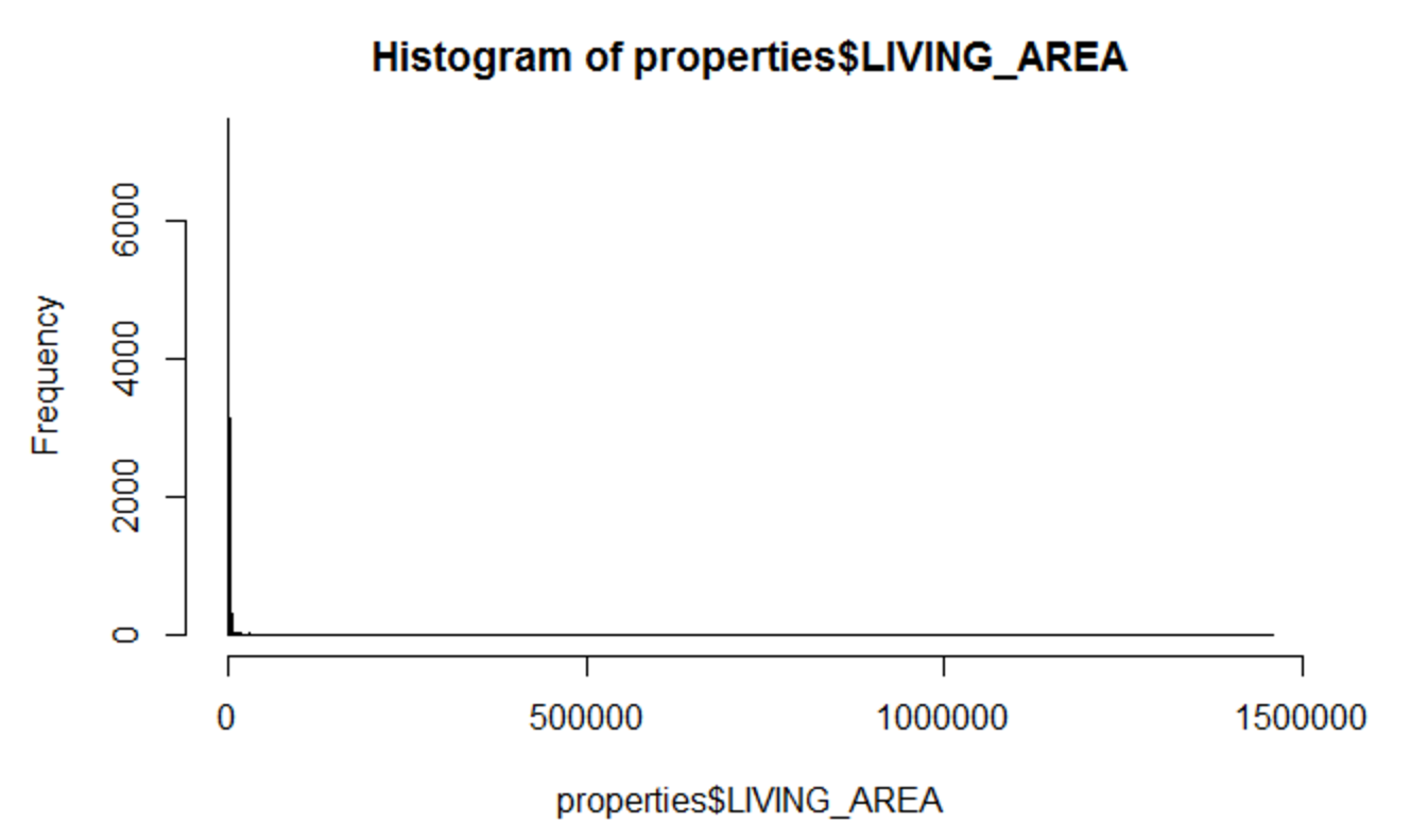
A quick google search of what that property is reveals that we're looking at the parking deck for the TD Garden... The weird thing is that it is listed as a land use of A which stands for: "Residential 7 or more units". If we look at the histogram of square footage we find the follwing:

hist(properties$LIVING_AREA, breaks= seq(0, ((max(properties$LIVING_AREA)%/%100)+1)*100, 100))
hist(properties[properties$LIVING_AREA < 20000, ]$LIVING_AREA, breaks= seq(0, 20000, 100))

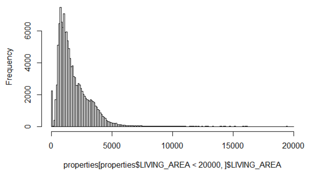
As would be expected the bulk of properties we have left in the data are between 100 and 5,000 square feet. For simplicity I will trim the data to only include things larger than 250 square feet (assumed to be a data error) and things less than 5,000 square feet.

nrow(properties)
properties <- properties[properties$LIVING_AREA > 250 & properties$LIVING_AREA <= 5000, ]
nrow(properties)

After cleaning out those oddly sized properties I only lost about ~5,000 records and now have a total of 124,000 (down from my original set of nearly 170k). In order to visualize these on a map I need the latitude and longitude values in the data to be accurate as well. Are there any with missing latitude or longitude values? The data read these values in as factors so first I need to convert them to numeric.

properties$LONGITUDE2 <- as.numeric(as.character(properties$LONGITUDE))
properties$LATITUDE2 <- as.numeric(as.character(properties$LATITUDE))

summary(properties$LONGITUDE2)
summary(properties$LATITUDE2)

Converting these values to numeric turned almost half of the records values into NA's. Look at a few examples of where this happened to see if I did something wrong.

head(properties[is.na(properties$LONGITUDE2), c("LATITUDE", "LONGITUDE", "LATITUDE2", "LONGITUDE2")])

Bummer, looks like a ton of the properties have missing lat/lon values. Double check that this is actually what happened throughout the other records.

nrow(properties[properties$LATITUDE=="#N/A", ])
nrow(properties[properties$LONGITUDE=="#N/A", ])

Confirmed that this is what happened. Maybe I can generate the lat/lon values on these properties using their street addresses. Try the first record with and #NA in the lat and lon values. Does it have a valid street address?

head(properties[properties$LATITUDE == "#N/A", c("ST_NUM", "ST_NAME", "ST_NAME_SUF", "UNIT_NUM", "ZIPCODE")])

There is a limit on the Google geocoding API of 2,500 per day. But it actually look like a lot of this data is the same street address and the various units within a particular building. To maximize the amount of geocoding we can do in a single day I can create a dataframe with just the unique street number and names to batch geocode them.

geocode.properties <- unique(properties[is.na(properties$LATITUDE2) | is.na(properties$LONGITUDE), c("ST_NUM", "ST_NAME", "ST_NAME_SUF", "ZIPCODE")])
nrow(geocode.properties)

There are only about 12,600 unique street addresses for the ~60k properties with missing lat/lon data. It will still take 5+ days to get all of these addresses geocoded, but that's better than the month it would have taken otherwise! For today I will geocode the top 2,500 properties based on the number of units they have. Basically, if I can get a buildings lat/lon that has 50 units I'd rather do that than a building with 2 units. At least to start.

require(sqldf)
geocode.properties <- sqldf("select ST_NUM, ST_NAME, ST_NAME_SUF, ZIPCODE, count(*) as Freq
                            from properties where LATITUDE = '#N/A' group by ST_NUM, ST_NAME, ST_NAME_SUF, ZIPCODE")
geocode.properties <- geocode.properties[order(geocode.properties$Freq, decreasing = TRUE), ]
geocode.properties$number <- 1:nrow(geocode.properties)

Now that the properties are in the right order, go through the top 2,500 and have them geocoded.

geocode.properties$Lat <- NA
geocode.properties$Lon <- NA

for(i in c(1:500)){
  temp <- geocode(paste0(as.character(geocode.properties[geocode.properties$number ==i, c("ST_NUM")]), " ", as.character(geocode.properties[geocode.properties$number ==i, c("ST_NAME")]), " ", as.character(geocode.properties[geocode.properties$number ==i, c("ST_NAME_SUF")]), ", Boston, MA"), messaging = FALSE)

  geocode.properties[geocode.properties$number==i, c("Lat")]<- temp$lat
  geocode.properties[geocode.properties$number==i, c("Lon")]<- temp$lon
}

Now that We have at least some of the missing lat/lon values that should be in this data -- merge it back to the original data source. First split out the original data into that with lat/lon data and that without. Add the new lat/lon data that we have then concatenate the two dataframes back together. Finally we need to create the dollars per square footage metric so that we can compare properties.

with.geo <- properties[!(properties$LATITUDE == "#N/A"| properties$LONGITUDE == "#N/A"), ]
without.geo <- properties[(properties$LATITUDE == "#N/A" | properties$LONGITUDE == "#N/A"), ]

without.geo <- sqldf("select a.*, b.Lat, b.Lon from `without.geo`as a left join `geocode.properties` as b on a.ST_NUM= b.ST_NUM and a.ST_NAME=b.ST_NAME and a.ST_NAME_SUF= b.ST_NAME_SUF and a.ZIPCODE=b.ZIPCODE")

without.geo$Lat <- as.numeric(as.character(without.geo$Lat))
without.geo$Lon <- as.numeric(as.character(without.geo$Lon))

without.geo$LATITUDE2 <- without.geo$Lat
without.geo$LONGITUDE2 <- without.geo$Lon

without.geo$Lat <- NULL
without.geo$Lon <- NULL

properties.final <- rbind.data.frame(with.geo, without.geo)

Finally take a look at the dollar values that are provided for the properties in this dataset.

summary(properties.final$AV_TOTAL)

There are only a few outrageously valued properties and after googling some it looks like a handful are actual penthouses while others are entire building values. To make things quick and easy I'm going to remove any properties that have a value of more than $7.5M and anything less than $100k.

properties.final <- properties.final[properties.final$AV_TOTAL>= 100000 & properties.final$AV_TOTAL<= 7500000, ]
properties.final$Dollars_per_SqFt <- properties.final$AV_TOTAL/properties.final$LIVING_AREA

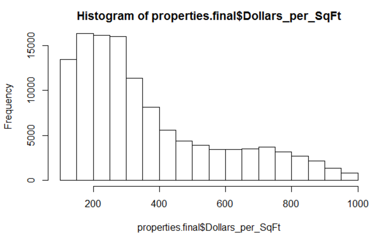
There are still some properties with wild dollars per sq. foot valuations. I'm talking more than $50k per sq foot. Quickly going to cut out properties that are valued more than $1,000 per sq foot.

properties.final <- properties.final[properties.final$Dollars_per_SqFt< 1000 & properties.final$Dollars_per_SqFt>=100, ]
nrow(properties.final)
hist(properties.final$Dollars_per_SqFt)

Now that we're done prepping the data set, take a look at these properties over a map of Boston.

base.map <- ggmap(get_map('Boston, Massachusetts',
                       zoom=12,
                       source='google',
                       maptype='terrain'))
boston.prop.box <- make_bbox(properties.final$LONGITUDE2, properties.final$LATITUDE2, f = 0.01)
map <- ggmap(get_map(boston.prop.box))

map +  
  geom_jitter(data= properties.final ,aes(x=LONGITUDE2, y=LATITUDE2,
             color = Dollars_per_SqFt), alpha=.15,size=1.2) +
  scale_color_gradientn(colours=rev(brewer.pal(10,"Spectral")))

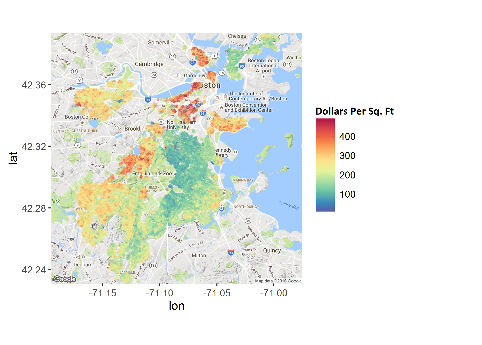
No surprises here, the South End and Back Bay are crazy expensive. Plenty of properties that are close to $1,000 per square foot. The North End also has some high prices, likely due to the tiny apartments that still have pretty significant price tags. What I think is more interesting is the string of more expensive places that seem to follow the Orange line out towards Jamaica Plain. I'm also surprised at how expensive the Allston properties are.

Dorchester and East Boston are the neighborhoods where you can get the most for your money but what is clear is that while the value of property has been on the rise in many Boston neighborhoods and surrounding areas (Cambridge and Somerville) -- these neighborhoods are somehow not seeing those benefits.

If you're interested in the code itself, I've pushed the R notebook to my github here: Boston Properties R Notebook